Article availability
Anna Krystalli
2017-10-21
Last updated: 2017-11-14
Code version: 29100a6
Session information
sessionInfo()R version 3.4.2 (2017-09-28)
Platform: x86_64-apple-darwin15.6.0 (64-bit)
Running under: macOS Sierra 10.12.6
Matrix products: default
BLAS: /Library/Frameworks/R.framework/Versions/3.4/Resources/lib/libRblas.0.dylib
LAPACK: /Library/Frameworks/R.framework/Versions/3.4/Resources/lib/libRlapack.dylib
locale:
[1] en_GB.UTF-8/en_GB.UTF-8/en_GB.UTF-8/C/en_GB.UTF-8/en_GB.UTF-8
attached base packages:
[1] stats graphics grDevices utils datasets methods base
loaded via a namespace (and not attached):
[1] compiler_3.4.2 backports_1.1.0 magrittr_1.5 rprojroot_1.2
[5] tools_3.4.2 htmltools_0.3.6 yaml_2.1.14 Rcpp_0.12.12
[9] stringi_1.1.5 rmarkdown_1.6 knitr_1.16 git2r_0.19.0
[13] stringr_1.2.0 digest_0.6.12 evaluate_0.10.1Load data
All article level data associated with the target publications where extracted from the sources table of the database and saved separately.
target_subset <- read_csv("../data/target_subset.csv")Parsed with column specification:
cols(
textID = col_integer(),
ID = col_integer(),
date = col_date(format = ""),
country = col_character(),
source = col_character(),
url = col_character(),
textTitle = col_character()
)Check unique source - country combinations
target_subset %>% select(source, country) %>% unique() %>% knitr::kable()| source | country |
|---|---|
| Daily Mail | GB |
| The Guardian | GB |
| The Guardian | US |
| The Guardian | IN |
| The Guardian | AU |
| The Guardian | NG |
| The Guardian | KE |
| The Guardian | CA |
| The Independent | GB |
| The Independent | US |
| The Independent | SG |
| Financial Times | GB |
| Financial Times | US |
| Independent | GB |
| Metro | GB |
| Evening Standard | GB |
| The National | GB |
| Daily Star | GB |
| The Courier | GB |
| The Courier | AU |
| The Courier | US |
| The Sun | GB |
| The Times | CA |
| The Atlantic | US |
| TIME | US |
| TIME | IN |
| TIME | PH |
| TIME | SG |
| TIME | CA |
| TIME | IE |
| TIME | AU |
| TIME | BD |
| Los Angeles Times | US |
| Wall Street Journal | US |
| Wall Street Journal | IN |
| Wall Street Journal | CA |
| Wall Street Journal | HK |
| Chicago Tribune | US |
| New York Daily News | US |
| Washington Post | US |
| New York Post | US |
| The Seattle Times | US |
| Washington Times | US |
| Washington Times | BD |
| Dallas Morning News | US |
| National Geographic | US |
| The Week Magazine | US |
| Baltimore Sun | US |
| The New Yorker | US |
| New York Magazine | US |
| Milwaukee Journal Sentinel | US |
| Minneapolis Star Tribune | US |
| Politico | US |
It appears that a number of target sources publish across many countries.
Q: Can you confirm whether you want only UK & US and how to handle sources across both? (see issue #6 for more details and discussion)
custom functions
# Multiple plot function
#
# ggplot objects can be passed in ..., or to plotlist (as a list of ggplot objects)
# - cols: Number of columns in layout
# - layout: A matrix specifying the layout. If present, 'cols' is ignored.
#
# If the layout is something like matrix(c(1,2,3,3), nrow=2, byrow=TRUE),
# then plot 1 will go in the upper left, 2 will go in the upper right, and
# 3 will go all the way across the bottom.
#
multiplot <- function(..., plotlist=NULL, file, cols=1, layout=NULL) {
library(grid)
# Make a list from the ... arguments and plotlist
plots <- c(list(...), plotlist)
numPlots = length(plots)
# If layout is NULL, then use 'cols' to determine layout
if (is.null(layout)) {
# Make the panel
# ncol: Number of columns of plots
# nrow: Number of rows needed, calculated from # of cols
layout <- matrix(seq(1, cols * ceiling(numPlots/cols)),
ncol = cols, nrow = ceiling(numPlots/cols))
}
if (numPlots==1) {
print(plots[[1]])
} else {
# Set up the page
grid.newpage()
pushViewport(viewport(layout = grid.layout(nrow(layout), ncol(layout))))
# Make each plot, in the correct location
for (i in 1:numPlots) {
# Get the i,j matrix positions of the regions that contain this subplot
matchidx <- as.data.frame(which(layout == i, arr.ind = TRUE))
print(plots[[i]], vp = viewport(layout.pos.row = matchidx$row,
layout.pos.col = matchidx$col))
}
}
}
# extract and save time-period word subsets
extract_tp_words <- function(date_subset, time_period, db, save_dir = "../data/") {
if(any(dbListTables(db) == "tp_subset")){dbRemoveTable(db, "tp_subset")}
dbWriteTable(db, "tp_subset", date_subset)
word_subset <- dbGetQuery(db, "select corpus.* , country, source
from tp_subset inner join corpus on corpus.textID = tp_subset.textID;")
save(word_subset, date_subset, time_period, file = paste0(save_dir, time_period,"-subset_data.RData"))
dbRemoveTable(db, "tp_subset")
}
# Plot descriptive statistics on article availability for time periods
time_period_desc_stats <- function(time_period, load_dir = "../data/"){
library(ggplot2)
library(grid)
library(gridExtra)
library(yarrr)
detach("package:tidyverse", unload=TRUE)
library(plyr)
library(tidyverse)
freqs <- function(by_group = "word") {
tab <- get(paste0(by_group, "_subset")) %>% select(source, country) %>% table %>% as.tibble() %>%
filter(n > 0) %>% arrange(source, desc(n))
# calculate cumulative sums for sorting
freqs_df <- ddply(tab, "source",
transform, label_ypos=cumsum(n)) %>%
arrange(label_ypos, source)
freqs_df$source <- factor(freqs_df$source, levels = unique(freqs_df$source))
return(freqs_df)
}
# get word count by textID (article)
textID_wc <- function(word_subset) {
word_subset %>% count("textID") %>% left_join(unique(select(word_subset, source, country, textID)), by = "textID")
}
# news-scrape pirate plots
news_scrape_pp <- function(formula, df, pal, main) {
pirateplot(as.formula(formula), df, pal = pal, main = main, theme = 4,
point.pch = 16,
point.o = .4,
point.col = pal,
point.bg = "white",
inf.b.o = 0.2,
inf.f.o = 0.3,
bean.f.o = .4, # Light bean filling
bean.b.o = .2,
hdi.o = .6,
bar.f.o = .1,
bar.f.col = pal,
avg.line.o = .5,
avg.line.col= pal)
}
# plot source level article word count data
word_pirate_plot <- function(word_subset, pal) {
# mode function
Mode <- function(x) {
ux <- unique(x)
ux[which.max(tabulate(match(x, ux)))]
}
# frequency table
freqs_by_source <- textID_wc(word_subset) %>% dplyr::group_by(source)
levels <- freqs_by_source %>% dplyr::summarise(mean = mean(freq)) %>% arrange(mean) %>% select(source) %>% unlist()
freqs_by_source$source <- factor(freqs_by_source$source,
levels = levels)
# country palette table
pals <- freqs_by_source %>% dplyr::summarise(mode = Mode(country))
pals$source <- factor(pals$source, levels = levels)
pals <- pals %>% arrange(source) %>% mutate(pal = case_when(mode == "GB" ~ pal[1],
TRUE ~ pal[2]))
x_lab_max <- max(4.1,max(nchar(as.character(freqs_by_source$source)))/1.8)
par(las = 2, mar = c(x_lab_max, 4, 4, 2), mgp = c(x_lab_max - 3 , 1, 0))
pirateplot(freq ~ source, freqs_by_source, pal = pals$pal, main = "distribution of word n across articles in target sources", theme = 4,
point.pch = 16,
point.o = .2,
point.col = pals$pal,
point.bg = "white",
inf.b.o = 0.2,
inf.f.o = 0.3,
bean.f.o = .4, # Light bean filling
bean.b.o = .2,
hdi.o = .6,
bar.f.o = .1,
bar.f.col = pals$pal,
avg.line.o = .5,
avg.line.col= pals$pal)
par(las = 2, mar = c(5, 4, 4, 2), mgp = c(3 , 1, 0))
}
load(file = paste0(load_dir, time_period,"-subset_data.RData"))
freqs_word <- freqs(by_group = "word")
freqs_date <- freqs(by_group = "date")
# source plot
p1 <- ggplot(data=freqs_date, aes(x=source, y=n, fill=country)) +
geom_bar(stat="identity")+ ggtitle("total article count per source") +
theme_minimal() + coord_flip()
pal <- ggplot_build(p1)$data[[1]]$fill %>% unique() %>% rev
p2 <- ggplot(data=freqs_word, aes(x=source, y=n, fill=country)) +
geom_bar(stat="identity")+ ggtitle("total word count per source") +
theme_minimal() + coord_flip()
multiplot(p1, p2, cols = 1, layout = matrix(c(1,1,1,1,1,1,1,1,1, 2,2,2,2,2,2,2,2)))
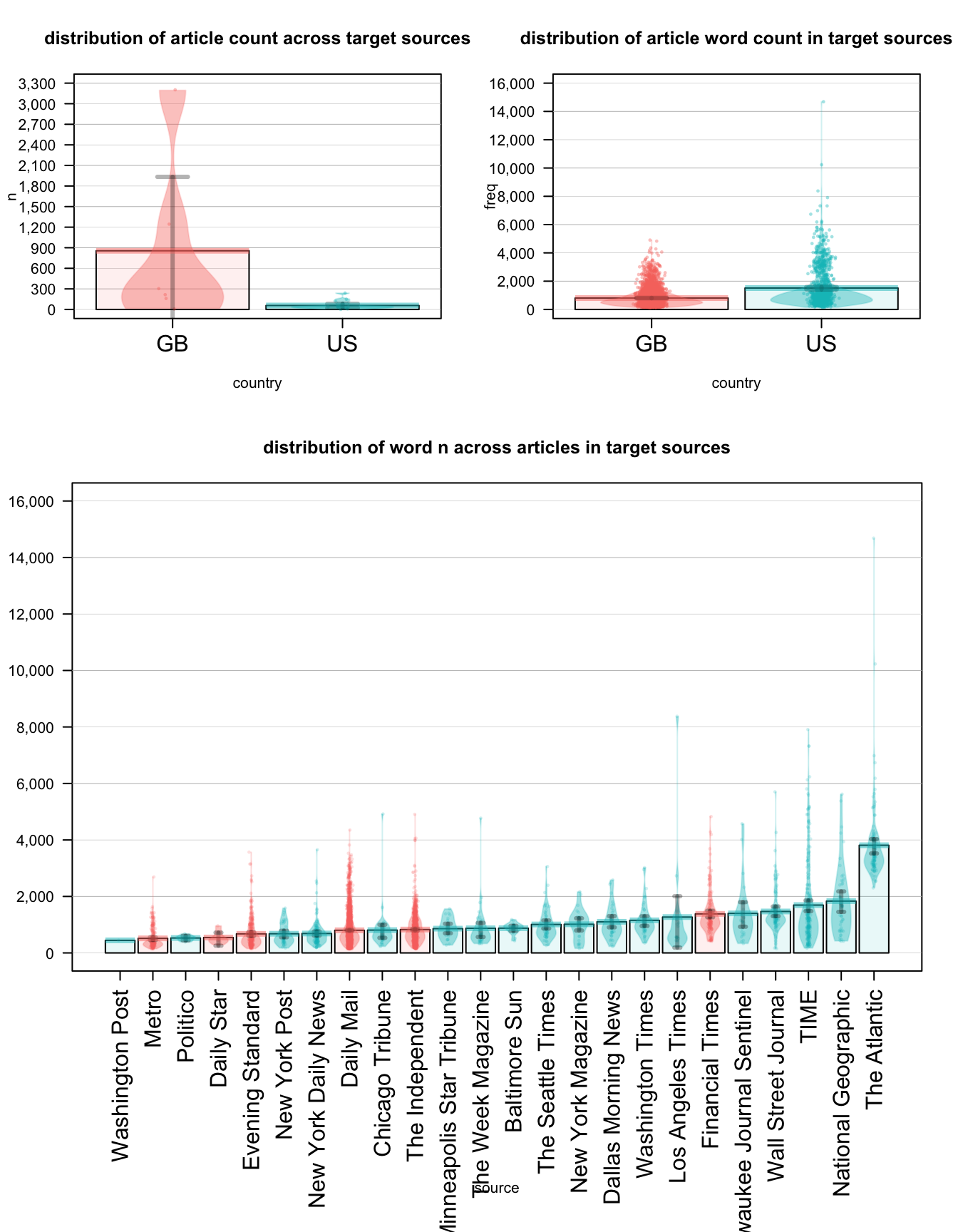
# pirate plot
layout(matrix(c(1,2,
1, 2,
1, 2,
3, 3,
3, 3,
3, 3), 6, 2, byrow = TRUE),
widths=c(2,2), heights=c(3,3,3,6,6,6))
news_scrape_pp(formula = "n ~ country", freqs_date, pal, main = "distribution of article count across target sources")
article_wc <- textID_wc(word_subset)
news_scrape_pp(formula = "freq ~ country", article_wc, pal, main = "distribution of article word count in target sources")
word_pirate_plot(word_subset, pal)
}Connect to database
#db <- dbConnect(RSQLite::SQLite(), dbname = "~/../../Volumes/ooominds1/Shared/corpus.byu.edu/a1517_now/now_db")
db <- dbConnect(RSQLite::SQLite(), dbname = "~/../../Volumes/ooominds1/User/ac1adk/now_db")
Extract word count data
Please note that this is the full word count (ie not unique word count and includes all stop words)
Also not all sources are represented during the two timeperiods of interest!
- e.g no guardian articles during the US election.
US ELECTION
target_subset %>% filter(date > "2012-10-08" & date < "2012-12-09" & country %in% c("GB", "US")) %>% mutate(time_period = "us_elec") %>% extract_tp_words(time_period = "use", db)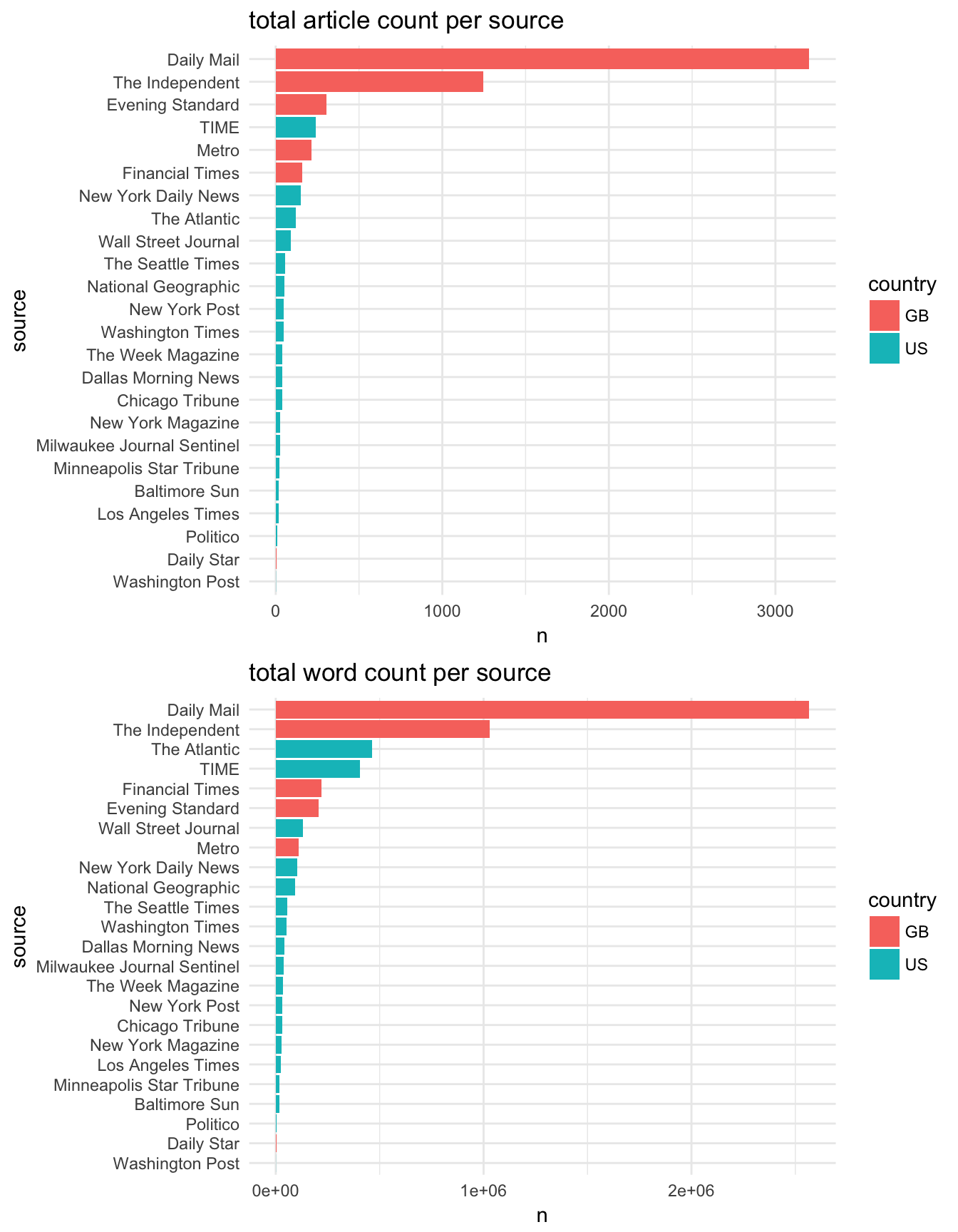
BREXIT
target_subset %>% filter(date > "2016-05-23" & date < "2016-07-24" & country %in% c("GB", "US")) %>% mutate(time_period = "brexit") %>% extract_tp_words(time_period = "brx", db)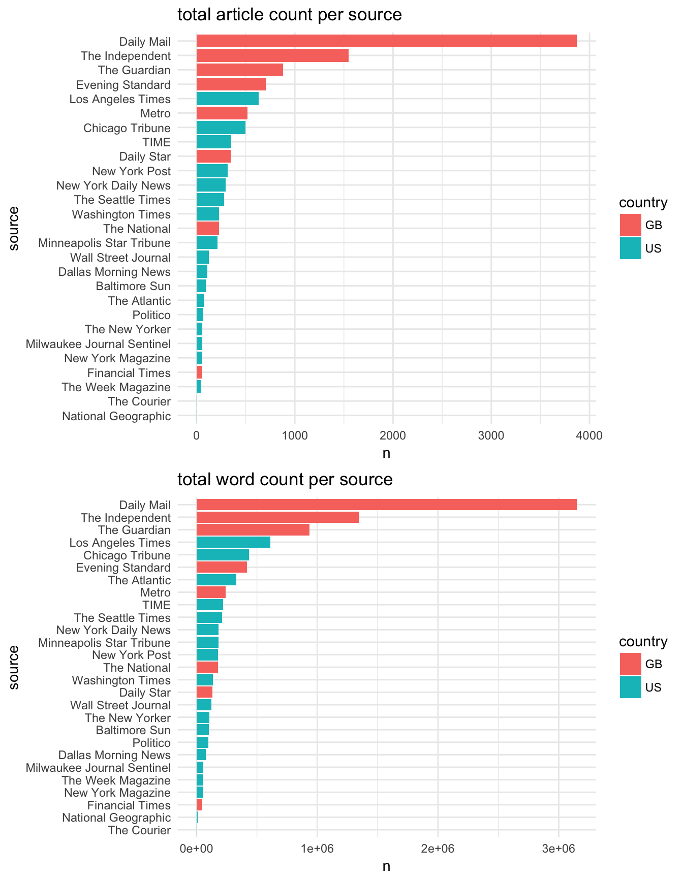
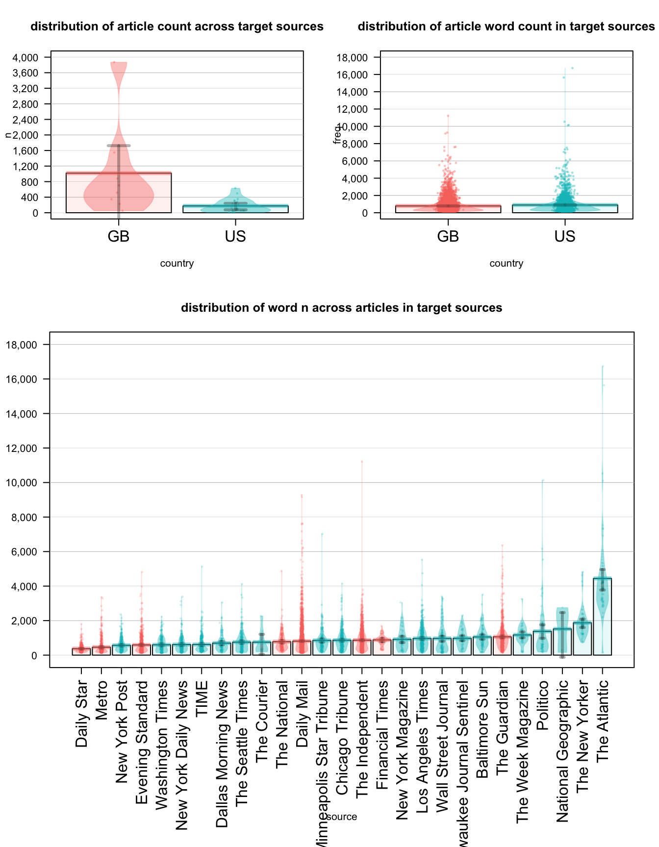
note on pirate plots
A pirateplot, is the RDI (Raw data, Descriptive statistics, and Inferential statistics) plotting choice of R pirates who are displaying the relationship between 1 to 3 categorical independent variables, and one continuous dependent variable.
A pirateplot has 4 main elements
- points, symbols representing the raw data (jittered horizontally)
- bar, a vertical bar showing central tendencies
- bean, a smoothed density (inspired by Kampstra and others (2008)) representing a smoothed density
- inf, a rectangle representing an inference interval (e.g.; Bayesian Highest Density Interval or frequentist confidence interval)
This R Markdown site was created with workflowr