Creating a research compendium with rrtools

Background

• Research is increasingly computational

• Code and data are important research outputs

  • yet, we still focus mainly on curating papers.

• Calls for openness

  • stick: reproducibility crisis
  • carrot: huge rewards from working open

Yet we lag in conventions and technical infrastructure for such openness.

Enter the Research Compendium

The goal of a research compendium is to provide a standard and easily recognizable way for organizing the digital materials of a project to enable others to inspect, reproduce, and extend the research.

Three Generic Principles

1. Organize its files according to prevailing conventions:

   • help other people recognize the structure of the project,
   • supports tool building which takes advantage of the shared structure.

2. Separate of data, method, and output, while making the relationship between them clear.

3. Specify the computational environment that was used for the original analysis.

R community response

R packages can be used as a research compendium for organising and sharing files!

R package file system structure for reproducible research

• Take advantage of the power of convention.

• Make use of great package development tools.

See Ben Marwick, Carl Boettiger & Lincoln Mullen (2018) Packaging Data Analytical Work Reproducibly Using R (and Friends), The American Statistician, 72:1, 80-88, DOI: <10.1080/00031305.2017.1375986>

images: Kartik Ram: rstudio::conf 2019 talk

Example use of the R package structure for a research compendium (source Marwick et al, 2018)

---

General Project Organisation

Good project layout helps ensure the

• Integrity of data
• Portability of the project
• Easier to pick the project back up after a break

---

From raw to analytical data

the reproducible pipeline

• Do not manually edit raw data

• Keep a clean pipeline of data processing from raw to analytical.

• Ideally, incorporate checks to ensure correct processing of data through to analytical.

• Check out rOpenSci package drake, an R-focused pipeline toolkit for reproducibility

---

Separate function definition and application

• When your project is new and shiny, the script file usually contains many lines of directly executated code.

• As it matures, reusable chunks get pulled into their own functions.

• The actual analysis scripts then become relatively short, and use the functions defined in separate R scripts.

---

Use Rstudio projects

Keep your work tidy, portable and self-contained

pkg here

Use function here::here("path", "to", "file") to create robust paths relative to the project root.

eg

here::here("path", "to", "file")

## [1] "/Users/runner/work/rrresearchACCE20/rrresearchACCE20/path/to/file"

---

Follow convention

It’s like agreeing that we will all drive on the left or the right. A hallmark of civilization is following conventions that constrain your behavior a little, in the name of public safety.

Jenny Bryan on Project-oriented workflows

A place for everything, everything in its place.

Benjamin Franklin

The benefits of following convention:

• You will be able to find your way around any of your projects

• You will be able to find your way around any project by others following same convention

• You will be able to find your way around any r package on GitHub!

---

R Developer Tools

Leverage tools and functionality for R package development

• manage dependencies
• make functionality available
• document functionality
• validate functionality
• version contol your project

devtools, usethis, rrtools, Rstudio

minimal analysis project

1. An scripts/ directory that contains R scripts (.R), notebooks (.Rmd), and intermediate data.

2. A DESCRIPTION file that provides metadata about the compendium. Most importantly, it would list the packages needed to run the analysis. Would contain field to indicate that this is an analysis, not a package.

A reproducible analysis project would also contain:

1. An R/ directory which contains R files that provide high-stakes functions.

2. A data/ directory which contains high-stakes data.

3. A tests/ directory that contains unit tests for the code and data.

4. A vignettes/ directory that contains high-stakes reports.

Autogenerated components:

1. A man/ directory which contains roxygen2-generated documentation for the reusable functions and data.

2. Online documentation in a docs/ folder.

A shareable reproducible analysis project would also:

• Use Git + GitHub (or other public Git host)

• Use Travis or other continuous integration service

• Capture the computational environment so it can easily be recreated on a different computer. This involves at a minimum capturing package versions, but might also include capturing R version, and other external dependencies.

Start small and build as necessary

images: Kartik Ram: rstudio::conf 2019 talk

---

rrtools: Research Compendia in R

The goal of rrtools is to provide instructions, templates, and functions for making a basic compendium suitable for writing reproducible research with R.

rrtools build on tools & conventions for R package development to

• organise files
• manage dependencies
• share code
• document code
• check and test code

rrtools extends and works with a number of R packages:

• devtools: functions for package development

• usethis: automates repetitive tasks that arise during project setup and development

• bookdown: facilitates writing books and long-form articles/reports with R Markdown

---

💻 Workshop materials

Data

On github: https://github.com/annakrystalli/rrtools-wkshp-materials/

• click on Clone or download

• click on Download ZIP

• Unzip the file

---

Workshop aims and objectives

In this workshop we’ll use materials associated with a published paper (text, data and code) to create a research compendium around it.

By the end of the workshop, you should be able to:

• Be able to Create a Research Compendium to manage and share resources associated with an academic publication.

• Be able to produce a reproducible manuscript from a single rmarkdown document.

• Appreciate the power of convention!

Let’s dive in!

💻Create your first reproducible research compendium

Let’s go ahead and create our first reproducible research compendium!

To do this in Rstudio Cloud (which is a bit fiddlier) we will create a general project in which we will create our reproducible research compendium project. In general, creating a project within a project is bad practice and you should avoid this when working locally, but given the more restrictive nature of working in Rstudio Cloud, we will break this general best practice rule.

Copy rrtools Project

In our shared space click on the copy button next to the rrtools Project.

Click on Save a permanent copy. You now have a personal copy of the project.

Install packages

In our rrtools project, these packages should be pre-installed and be available to the research compendium we’ll create inside.

However, if you are working locally, you would need to install the following packages starting with rrtools (if you haven’t got devtools installed, you’ll need to before you can install rrtools from GitHub).

# install rrtools
install.packages("devtools")
devtools::install_github("benmarwick/rrtools")

# install github dependencies
dependencies <- c("dplyr", "ggplot2", "ggthemes", "gitcreds", "rticles", "Cairo")

# install CRAN dependencies
install.packages(dependencies)

#install github dependencies
devtools::install_github("crsh/citr")

# install tinytex
tinytex::install_tinytex()

Installing rrtools imports many of the packages we’ll need today (eg, have a look at the imports section of the DESCRIPTION file).

Imports: devtools, git2r, whisker, rstudioapi, rmarkdown, curl, RCurl, jsonlite, methods, httr,          usethis, clisymbols, crayon, glue, bookdown, here

We also install some additional packages we’ll need for the workshop.

You might also need to install tinytex (if you get errors when rendering your Rmd paper).

🚦 Create compendium

Now that we’ve got all the materials we need, let’s start by *creating a blank research compendium for us to work in.

load library

First we need to load rrtools

library(rrtools) 

## ✖ Git is installed on this computer, but not configured for use. For more information on configuring and using Git, see http://happygitwithr.com/

This performs a quick check to confirm you have Git installed and configured

If you do, you should see the following output in the console.

✔ Git is installed on this computer, your username is annakrystalli

create compendium

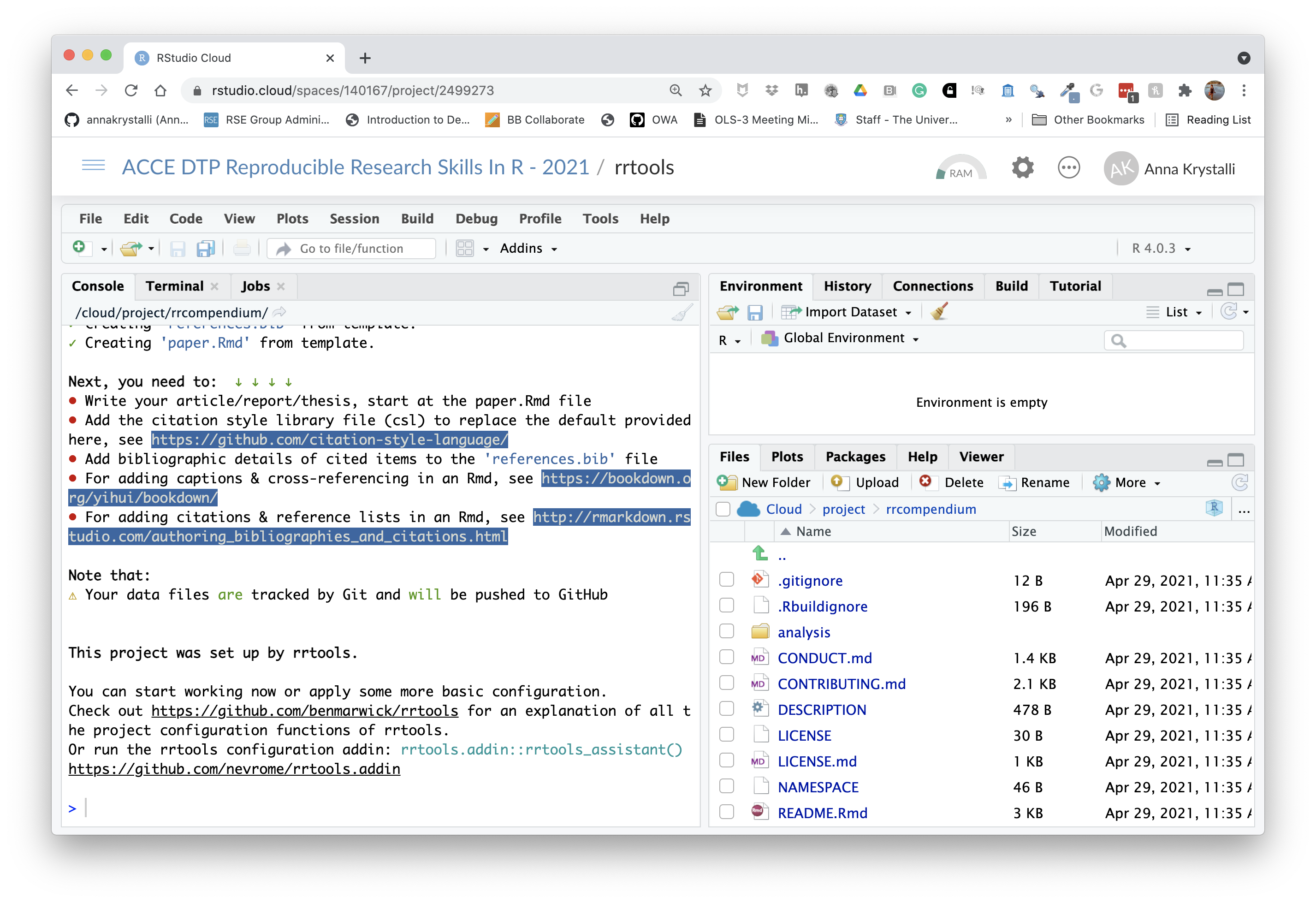
Now we’re ready to create our compendium. We use function rrtools::create_compendium and supply it with a path at which our compendium will be created. The final part of our path becomes the compendium name. Because the function effectively creates a package, only a single string of lowercase alpha characters is accepted as a name. so let’s go for rrcompendium as the final part of our path.

To create rrcompendium in our project, I use:

rrtools::create_compendium("rrcompendium")

If the call was successfull you should see the following console output:

✓ Setting active project to '/cloud/project/rrcompendium'
✓ Writing 'LICENSE'
✓ Writing 'LICENSE.md'
✓ Adding '^LICENSE\\.md$' to '.Rbuildignore'

✓ Creating 'README.Rmd' from template.
✓ Adding 'README.Rmd' to `.Rbuildignore`.
• Modify 
✓ Adding code of conduct.
✓ Creating 'CONDUCT.md' from template.
✓ Adding 'CONDUCT.md' to `.Rbuildignore`.
✓ Adding instructions to contributors.
✓ Creating 'CONTRIBUTING.md' from template.
✓ Adding 'CONTRIBUTING.md' to `.Rbuildignore`.
✓ Adding runtime.txt for Binder

✓ Adding 'bookdown' to Imports
✓ Adding 'here' pkg to Imports
✓ Creating 'analysis' directory and contents
✓ Creating 'analysis'
✓ Creating 'analysis/paper'
✓ Creating 'analysis/figures'
✓ Creating 'analysis/templates'
✓ Creating 'analysis/data'
✓ Creating 'analysis/data/raw_data'
✓ Creating 'analysis/data/derived_data'
✓ Creating 'analysis/supplementary-materials'
✓ Creating 'references.bib' from template.
✓ Creating 'paper.Rmd' from template.

Next, you need to:  ↓ ↓ ↓ ↓ 
• Write your article/report/thesis, start at the paper.Rmd file
• Add the citation style library file (csl) to replace the default provided here, see https://github.com/citation-style-language/
• Add bibliographic details of cited items to the 'references.bib' file
• For adding captions & cross-referencing in an Rmd, see https://bookdown.org/yihui/bookdown/
• For adding citations & reference lists in an Rmd, see http://rmarkdown.rstudio.com/authoring_bibliographies_and_citations.html

Note that:
⚠ Your data files are tracked by Git and will be pushed to GitHub 


This project was set up by rrtools.

You can start working now or apply some more basic configuration.
Check out https://github.com/benmarwick/rrtools for an explanation of all the project configuration functions of rrtools.
Or run the rrtools configuration addin: rrtools.addin::rrtools_assistant() https://github.com/nevrome/rrtools.addin

and a new Rstudio session launched for the compendium:

Initiate git

Let’s initialise our compendium with .git. We’ll need to configure git again as this is a new Rstudio cloud project.

# configure git
use_git_config(user.name = "Jane",
               user.email = "jane@example.org")
# intialise git and commit
usethis::use_git()

N.B. Beware, if you are working locally, you may have ended up with two Rstudio sessions of rrcompendium. Make sure to only have one session of a single project at one time to avoid problems.

Inspect templates

.
├── DESCRIPTION <- .............................package metadata
|                                               dependency management
├── NAMESPACE <- ...............................AUTO-GENERATED on build
├── R <- .......................................folder for functions
├── man <- .....................................AUTO-GENERATED on build
└── rrcompendium.Rproj <- ......................rstudio project file

rrtools::create_compendium() creates the bare backbone of infrastructure required for a research compendium. At this point it provides facilities to store general metadata about our compendium (eg bibliographic details to create a citation) and manage dependencies in the DESCRIPTION file and store and document functions in the R/ folder. Together these allow us to manage, install and share functionality associated with our project.

Get workshop materials

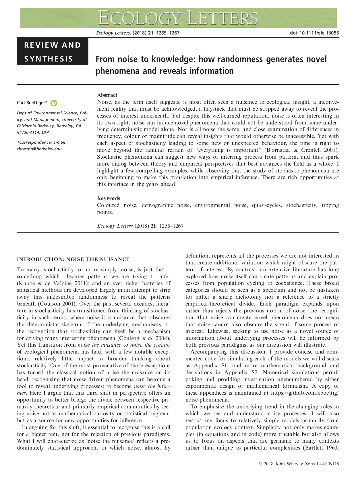
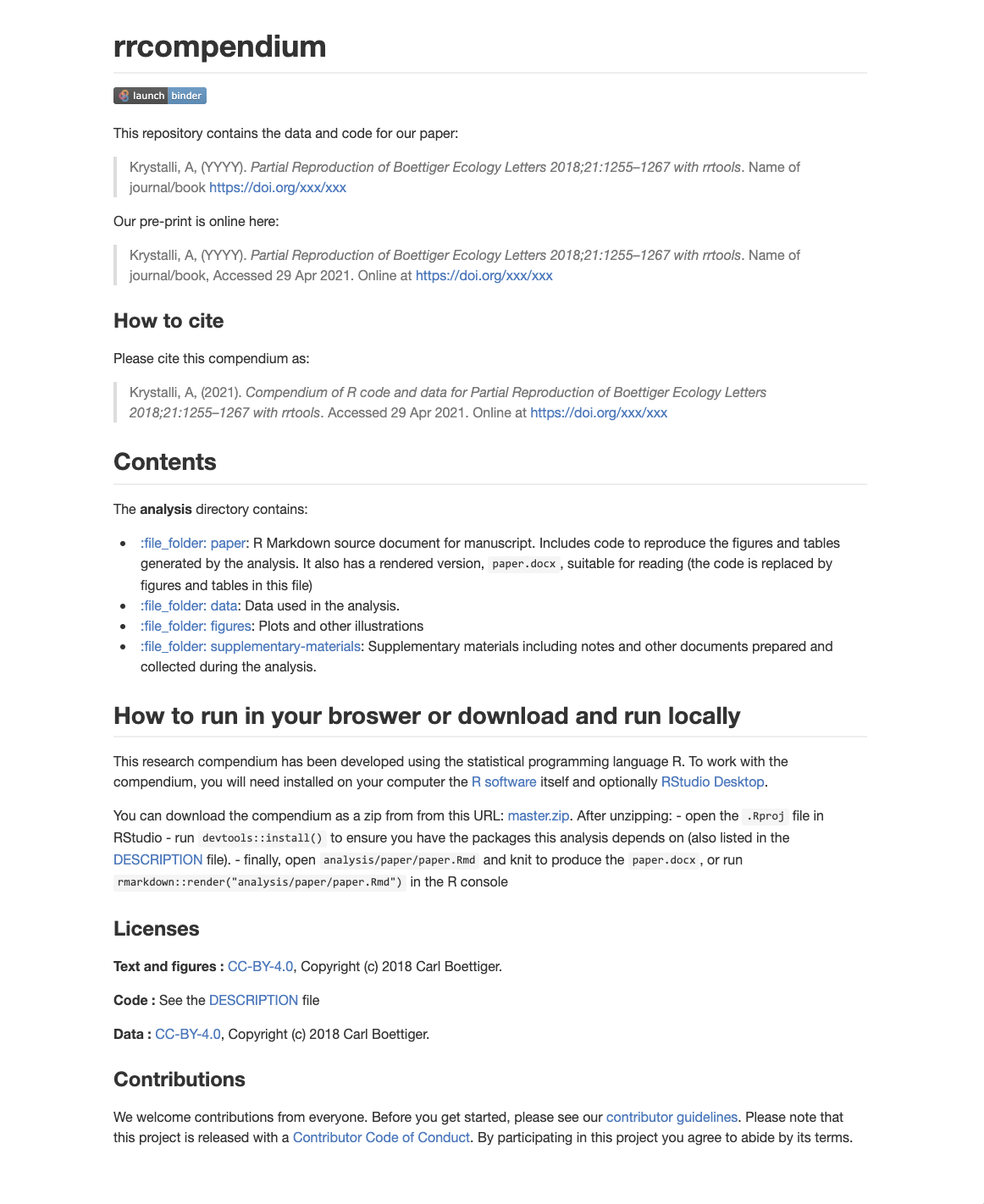
Today we’ll be working with a subset of materials from the published compendium of code, data, and author’s manuscript:

Carl Boettiger. (2018, April 17). cboettig/noise-phenomena: Supplement to: “From noise to knowledge: how randomness generates novel phenomena and reveals information” (Version revision-2). Zenodo. http://doi.org/10.5281/zenodo.1219780

accompanying the publication:

Carl Boettiger . From noise to knowledge: how randomness generates novel phenomena and reveals information. Published in Ecology Letters, 22 May 2018 https://doi.org/10.1111/ele.13085

Let’s first create a folder to dowload the materials into. It’s sometimes useful to have a folder to hold materials that are not formally part of the project (i.e. we will not commit these files to git). I like to call such folders attic, so let’s create such a folder

dir.create("attic")

Let’s also add the attic/ dir to .gitignore by adding the following text to it (remember to include a new line at the end of the file)

attic/*

You can download the materials using usethis::use_course() and supplying a path to a destination folder to argument destdir. Let’s download everything into the attic/ folder.

usethis::use_course(url = "bit.ly/rrtools_wks", destdir = "attic")

This will download everything we need from a GitHub repository as a .zip file, unzip it and launch it in a new Rstudio session for us to explore.

Inspect materials

The follwing files should now be contained in your attic/rrtools-wkshp-materials-master folder

├── README.md <- .......................repo README
├── analysis.R <- ......................analysis underlying paper
├── gillespie.csv <- ...................data
├── paper.pdf <- .......................LaTex pdf of the paper
├── paper.txt <- .......................text body of the paper
└── refs.bib <- ........................bibtex bibliographic file

In this workshop we’ll attempt a partial reproduction of the original paper using the materials we’ve just downloaded.

We’ll use this as an opportunity to create a new research compendium using rrtools and friends! 🎊

---

🚦 Update DESCRIPTION file

Let’s update some basic details in the DESCRIPTION file:

Package: rrcompendium
Title: What the Package Does (One Line, Title Case)
Version: 0.0.0.9000
Authors@R:
    person(given = "First",
           family = "Last",
           role = c("aut", "cre"),
           email = "first.last@example.com")
Description: What the package does (one paragraph).
License: MIT + file LICENSE
ByteCompile: true
Encoding: UTF-8
LazyData: true
Roxygen: list(markdown = TRUE)
RoxygenNote: 7.1.1
Imports: bookdown,
    here
Suggests: devtools,
    git2r

Title

Let’s start with giving our compendium a descriptive title:

Title: Partial Reproduction of Boettiger Ecology Letters 2018;21:1255–1267 
    with rrtools

Version

We don’t need to change the version now but using semantic versioning for our compendium can be a really useful way to track versions. In general, versions below 0.0.1 are in development, hence the DESCRIPTION file defaults to 0.0.0.9000.

Authors

Next let’s specify the author of the compendium. Edit with your own details.

Authors@R: 
    person(given = "Anna",
           family = "Krystalli",
           role = c("aut", "cre"),
           email = "annakrystalli@googlemail.com")

For more details on specifying authors, check documentation for ?person

Description

Let’s add a bit more detail about the contents of the compendium in the Description.

Description: This repository contains the research compendium of the 
    partial reproduction of Boettiger Ecology Letters 2018;21:1255–1267. 
    The compendium contains all data, code, and text associated with this       sub-section of the analysis

License

Finally, let’s create a new license for the material we create. We’ll use an MIT license. Note however that his only covers the code. We can do this with:

usethis::use_mit_license("Anna Krystalli")

✔ Setting License field in DESCRIPTION to 'MIT + file LICENSE'
✔ Writing 'LICENSE.md'
✔ Adding '^LICENSE\\.md$' to '.Rbuildignore'

This overwrites the current files LICENSE and LICENSE.md and updates the DESCRIPTION file, embedding our name in the details of the license.

License: MIT + file LICENSE

Recap

We’ve finished updating our DESCRIPTION file! 🎉

It should look a bit like this:

Package: rrcompendium
Title: Partial Reproduction of Boettiger Ecology Letters 2018;21:1255–1267 
    with rrtools
Version: 0.0.0.9000
Authors@R: 
    person(given = "Anna",
           family = "Krystalli",
           role = c("aut", "cre"),
           email = "annakrystalli@googlemail.com")
Description: This repository contains the research compendium of the partial 
    reproduction of Boettiger Ecology Letters 2018;21:1255–1267. The compendium 
    contains all data, code, and text associated with this sub-section of the 
    analysis.
License: MIT + file LICENSE
ByteCompile: true
Encoding: UTF-8
LazyData: true
Roxygen: list(markdown = TRUE)
RoxygenNote: 7.1.1
Imports: bookdown,
    here
Suggests: devtools,
    git2r

and your project folder should contain:

├── CONDUCT.md
├── CONTRIBUTING.md
├── DESCRIPTION
├── LICENSE
├── LICENSE.md
├── NAMESPACE
├── README.Rmd
├── analysis
│   ├── data
│   │   ├── DO-NOT-EDIT-ANY-FILES-IN-HERE-BY-HAND
│   │   ├── derived_data
│   │   └── raw_data
│   ├── figures
│   ├── paper
│   │   ├── paper.Rmd
│   │   └── references.bib
│   ├── supplementary-materials
│   └── templates
│       ├── author-info-blocks.lua
│       ├── journal-of-archaeological-science.csl
│       ├── pagebreak.lua
│       ├── scholarly-metadata.lua
│       ├── template.Rmd
│       └── template.docx
├── attic
│   └── rrtools-wkshp-materials-master
│       ├── README.md
│       ├── analysis.R
│       ├── gillespie.csv
│       ├── paper.pdf
│       ├── paper.txt
│       └── refs.bib
├── rrcompendium.Rproj
└── runtime.txt

Let’s commit our work and move on to preparing our compendium for sharing on GitHub.

---

🚦Sharing a compendium on GitHub

Update README

Every GitHub repository needs a README landing page.

When we intialised our research compendium, an rrtools README template was created.

You can always re-create one with:

rrtools::use_readme_rmd()

✔ Creating 'README.Rmd' from template.
✔ Adding 'README.Rmd' to `.Rbuildignore`.
● Modify 'README.Rmd'
✔ Rendering README.Rmd to README.md for GitHub.
✔ Adding code of conduct.
✔ Creating 'CONDUCT.md' from template.
✔ Adding 'CONDUCT.md' to `.Rbuildignore`.
✔ Adding instructions to contributors.
✔ Creating 'CONTRIBUTING.md' from template.
✔ Adding 'CONTRIBUTING.md' to `.Rbuildignore`.

This generates README.Rmd and renders it to README.md, ready to display on GitHub. It contains:

• details of authorship and DOI of the associated paper.
• details of authorship and DOI of the code and data.
• a template citation to show others how to cite your project.
• instructions on how to download and install the compendium
• instructions on how to reproduce the analysis
• license information for the text, figures, code and data in your compendium

The call also adds two other markdown files:

• CONDUCT.md: a code of conduct for users
• CONTRIBUTING.md:: basic instructions for people who want to contribute to our compendium

update README

There’s 4 main edits we need to make to the template:

add title

In the first code chunk, assign the title to the title object:

Title <- "Partial Reproduction of Boettiger Ecology Letters 2018;21:1255–1267 with rrtools"

edit author details

Where details of authors are requested, add your own name

We don’t have a link to the DOI or details of where our partial reproduction is published so just leave as is.

update zip url

This is a link to download a zipped file of the repository. To update the template, just paste the url of your compendium repository like so:

[master.zip](https://github.com/annakrystalli/rrcompendium/archive/master.zip)

adjust data LICENSE

Let’s adjust the data LICENSE to match the source compendium license, which is CC-BY 4.0. Let’s also add Carl Boettiger as copyright holder of the data.

**Text and figures :**  [CC-BY-4.0](http://creativecommons.org/licenses/by/4.0/), Copyright (c) 2018 Carl Boettiger.

**Code :** See the [DESCRIPTION](DESCRIPTION) file

**Data :** [CC-BY-4.0](http://creativecommons.org/licenses/by/4.0/), Copyright (c) 2018 Carl Boettiger.

Remember to knit your README.Rmd to it’s .md version.

🚦 Create GitHub repository

Next, we’ll create a GitHub repository to share our compendium. We’ll make use of our GITHUB_PAT and go for https authentication. We can do this with function:

You will need to set up gitcreds again in this new project!

# configure GitHub PAT credentials
gitcreds::gitcreds_set()

# create GitHub repository and push
usethis::use_github(protocol = "https")

✔ Setting active project to '/Users/Anna/Documents/workflows/rrcompendium'
● Check title and description
  Name:        rrcompendium
  Description: Partial Reproduction of Boettiger Ecology Letters 2018;21:1255–1267 with rrtools
  

The function will prompt you to confirm the name and description for your GitHub repo which it parses from our DESCRIPTION file. If everything looks good select the affirmative option.

Are title and description ok?
1: Not now
2: Definitely
3: Nope

If creation of the repo was successfull you should see the following console output:

✔ Creating GitHub repository
✔ Adding GitHub remote
✔ Adding GitHub links to DESCRIPTION
✔ Setting URL field in DESCRIPTION to 'https://github.com/annakrystalli/rrcompendium'
✔ Setting BugReports field in DESCRIPTION to 'https://github.com/annakrystalli/rrcompendium/issues'
✔ Pushing to GitHub and setting remote tracking branch
✔ Opening URL https://github.com/annakrystalli/rrcompendium

Commit and push to GitHub

We’ve now completed our rrtools README.Rmd! 🎉

• Render it to update the README.md file which is displayed on GitHub

• Commit and push to GitHub.

You’re Github repository README should look like this on the site:

---

---

🚦 Setting up the analysis folder

Complete analysis

We’ll now move to working in our analysis folder which will contain our analysis and paper. It already exists but you can re-create it by using function rrtools::use_analysis()

The function has three location = options:

• top_level to create a top-level analysis/ directory

• inst to create an inst/ directory (so that all the sub-directories are available after the package is installed)

• vignettes to create a vignettes/ directory (and automatically update the DESCRIPTION).

The default is a top-level analysis/.

rrtools::use_analysis()

✔ Adding bookdown to Imports
✔ Creating 'analysis' directory and contents
✔ Creating 'analysis'
✔ Creating 'analysis/paper'
✔ Creating 'analysis/figures'
✔ Creating 'analysis/templates'
✔ Creating 'analysis/data'
✔ Creating 'analysis/data/raw_data'
✔ Creating 'analysis/data/derived_data'
✔ Creating 'references.bib' from template.
✔ Creating 'paper.Rmd' from template.

Next, you need to:  ↓ ↓ ↓ ↓ 
● Write your article/report/thesis, start at the paper.Rmd file
● Add the citation style library file (csl) to replace the default provided here, see https://github.com/citation-style-language/
● Add bibliographic details of cited items to the 'references.bib' file
● For adding captions & cross-referencing in an Rmd, see https://bookdown.org/yihui/bookdown/
● For adding citations & reference lists in an Rmd, see http://rmarkdown.rstudio.com/authoring_bibliographies_and_citations.html

Note that:
⚠ Your data files are tracked by Git and will be pushed to GitHub

Regardless for location option, the contents of the created sub-directories are the same:

analysis
├── data
│   ├── DO-NOT-EDIT-ANY-FILES-IN-HERE-BY-HAND
│   ├── derived_data
│   └── raw_data
├── figures
├── paper
│   ├── paper.Rmd
│   └── references.bib
├── supplementary-materials
└── templates
    ├── author-info-blocks.lua
    ├── journal-of-archaeological-science.csl
    ├── pagebreak.lua
    ├── scholarly-metadata.lua
    ├── template.Rmd
    └── template.docx

Let’s inspect

paper.Rmd

paper.Rmd is ready to write in and render with bookdown. It includes:

• a YAML header that identifies the references.bib file and the supplied csl file (Citation Style Language) to style the reference list)

• a colophon that adds some git commit details to the end of the document. This means that the output file (HTML/PDF/Word) is always traceable to a specific state of the code.

references.bib

The references.bib file has just one item to demonstrate the format. It is ready to insert more reference details.

We can replace the supplied csl file with a different citation style from https://github.com/citation-style-language/

---

🚦 Reproduce a paper in Rmd

In this section we’re going to create a literate programming document to reproduce the paper in a format suitable for journal submission or as a pre-print. We’ll do this using the course materials we downloaded.

In particular, we’re going to combine the code in analysis.R, the text in paper.txt and the references in the refs.bib file in an .Rmd document to reproduce paper.pdf.

More information on working on academic journals with Bookdown

Setup data

Copy data to data/

To begin, let’s copy gillespie.csv from the course materials you downloaded in rrtools-wkshp-materials-master/ to the subfolder analysis/data/raw_data/ in rrcompendium

We can do this programmatically with:

fs::file_copy("attic/rrtools-wkshp-materials-master/gillespie.csv", 
              "analysis/data/raw_data/")

Your data folder should now look like this:

analysis/data
├── DO-NOT-EDIT-ANY-FILES-IN-HERE-BY-HAND
├── derived_data
└── raw_data
    └── gillespie.csv

Inspect analysis.R file

Let’s also open analysis.R in the course materials and run the code. The script has some initial setup, then loads the data, recodes one of the columns for plotting and then plots the results of the simulation, which generates figure 1 in paper.pdf.

analysis.R

library(dplyr)
library(readr)
library(ggplot2)
library(ggthemes)
theme_set(theme_grey())

# load-data
data <- read_csv(here::here("gillespie.csv"), col_types = "cdiddd")

# create colour palette
colours <- ptol_pal()(2)

# recode-data
data <- data %>% 
  mutate(system_size = recode(system_size, 
                              large = "A. 1000 total sites", 
                              small = "B. 100 total sites")) 

# plot-gillespie
data %>%
  ggplot(aes(x = time)) + 
  geom_hline(aes(yintercept = mean), lty=2, col=colours[2]) + 
  geom_hline(aes(yintercept = minus_sd), lty=2, col=colours[2]) + 
  geom_hline(aes(yintercept = plus_sd), lty=2, col=colours[2]) + 
  geom_line(aes(y = n), col=colours[1]) +
  facet_wrap(~system_size, scales = "free_y")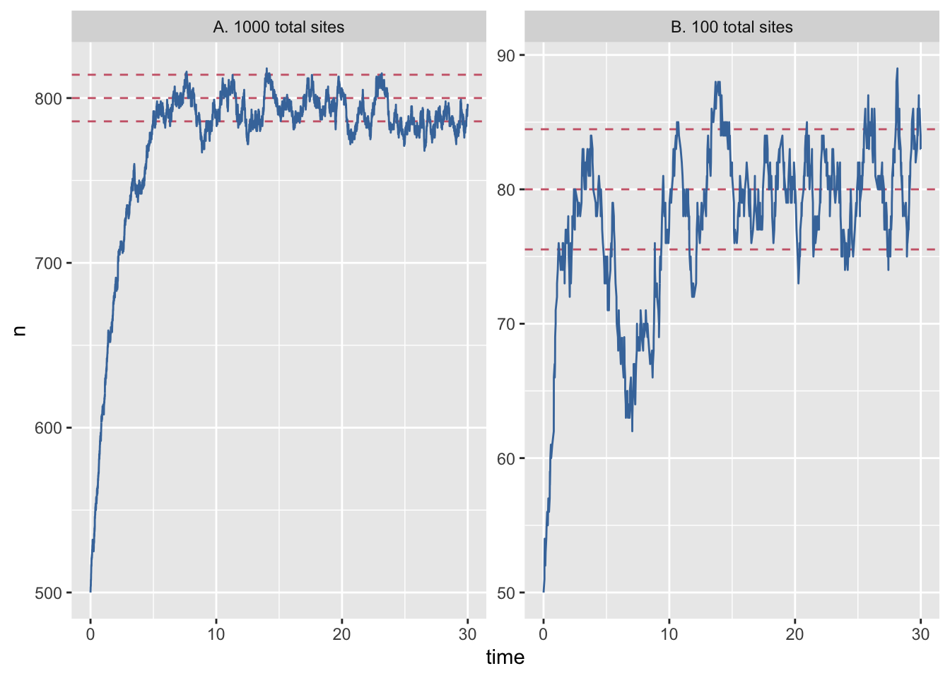 

---

🚦 Create journal article template using rticles

The rticles package is designed to simplify the creation of documents that conform to submission standards. A suite of custom R Markdown templates for popular journals is provided by the package.

delete paper/ subdirectory

First, let’s delete the current analysis/paper folder as we’re going to create a new folder and paper.Rmd template.

We can do this programmatically with:

fs::dir_delete("analysis/paper")

create new paper template

This particular paper was published in Ecology Letters, an Elsevier Journal. We can create a new paper.Rmd template from the templates provided by rticles package.

We can use the New R Markdown dialog

Select:

• Template: Elesevier Journal Article
• Name: paper
• Location: rrcompendium/analysis

knitr::include_graphics("assets/rticle.png")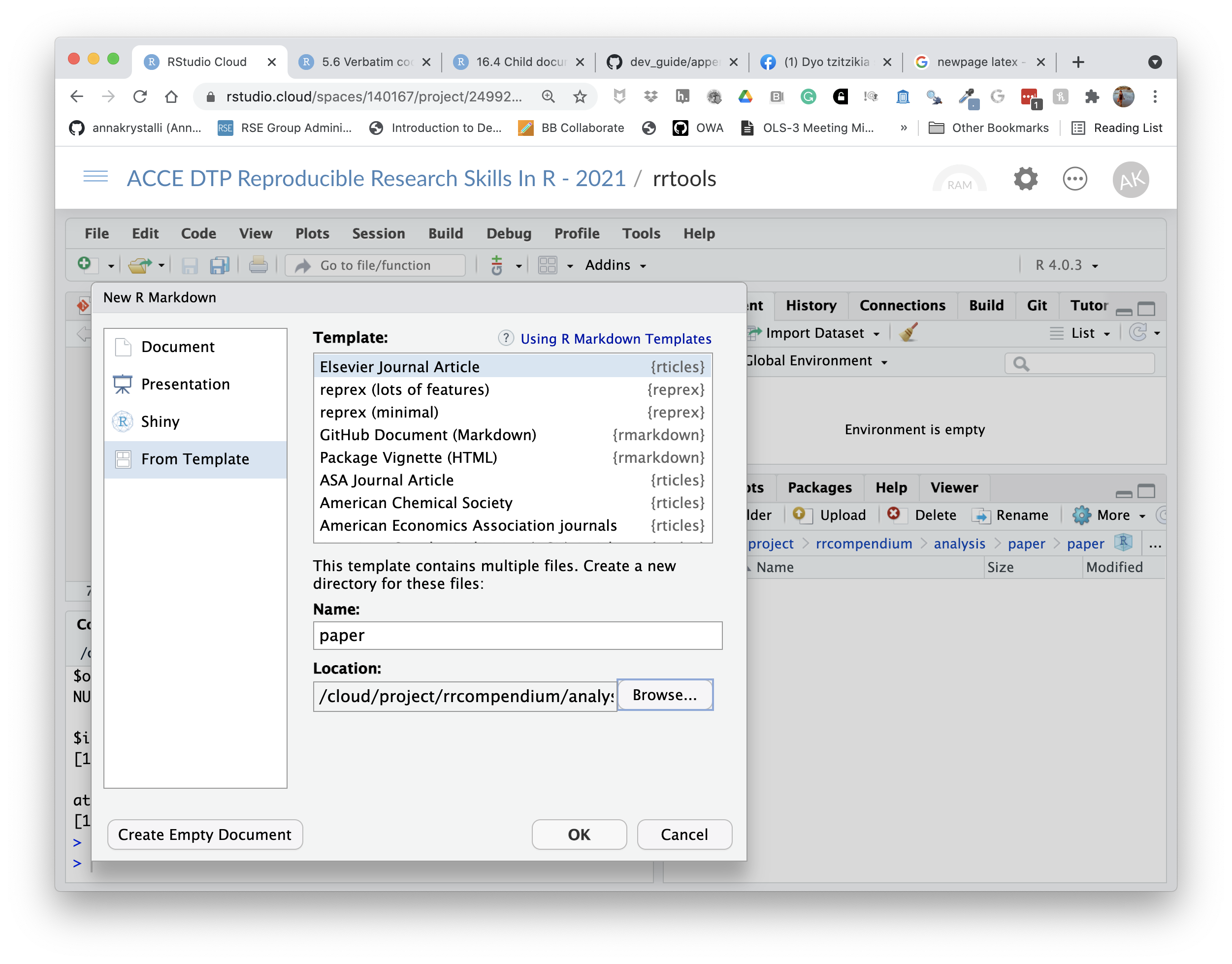

Or we can use rmarkdown::draft() to create articles:

rmarkdown::draft(here::here("analysis","paper.Rmd"), template = "elsevier", package = "rticles")

Both these functions create the following files in a new directory analysis/paper.

analysis/paper
├── elsarticle.cls
├── elsevier-harvard-without-titles.csl
├── elsevier-harvard.csl
├── elsevier-vancouver.csl
├── elsevier-with-titles-alphabetical.csl
├── elsevier-with-titles.csl
├── elsevier-without-titles.csl
├── mybibfile.bib
├── numcompress.sty
└── paper.Rmd

• The *.cls files contain citation language styles for the references.

• The mybibfile.bib contains an example reference list.

• The new paper.Rmd is the file we will be working in.

Let’s open it up and start editing it.

---

🚦 Update YAML

The YAML header in Paper.Rmd contains document wide metadata and is pre-populated with some fields relevant to an academic publication.

---
title: Short Paper
author:
  - name: Alice Anonymous
    email: alice@example.com
    affiliation: Some Institute of Technology
    footnote: 1
  - name: Bob Security
    email: bob@example.com
    affiliation: Another University
  - name: Cat Memes
    email: cat@example.com
    affiliation: Another University
    footnote: 2
  - name: Derek Zoolander
    email: derek@example.com
    affiliation: Some Institute of Technology
    footnote: 2
address:
  - code: Some Institute of Technology
    address: Department, Street, City, State, Zip
  - code: Another University
    address: Department, Street, City, State, Zip
footnote:
  - code: 1
    text: "Corresponding Author"
  - code: 2
    text: "Equal contribution"
abstract: |
  This is the abstract.

  It consists of two paragraphs.

journal: "An awesome journal"
date: "2022-01-18"
bibliography: mybibfile.bib
#linenumbers: true
#numbersections: true
csl: elsevier-harvard.csl
output: rticles::elsevier_article
---

Here we’re going to reproduce paper.pdf as is, so we’ll actually be editing the file with details from the original publication.

First, let’s clear all text BELOW the YAML header (which is delimited by ---. DO NOT delete the YAML header).

Next, let’s open paper.txt from the course material which contains all text from the in paper.pdf. We can use it to complete some of the fields in the YAML header.

title

Add the paper title to this field

title: "From noise to knowledge: how randomness generates novel phenomena and reveals information"

author

Here we specify author details.

author:
  - name: "Carl Boettiger"
    affiliation: a
    email: "cboettig@berkeley.edu"

address

Here we specify the addresses associated with the affiliations specified in authors

address:
  - code: a
    address: "Dept of Environmental Science, Policy, and Management, University of California Berkeley, Berkeley CA 94720-3114, USA"

Note that the field code in address cross-references with the affiliations specified in author.

bibliography

Before specifying the bibliography, we need to copy the refs.bib file associated with paper.pdf from the course materials and save it in our analysis/paper subdirectory.

We can do this programmatically with:

fs::file_copy("attic/rrtools-wkshp-materials-master/refs.bib", "analysis/paper/")

Next we can set the refs.bib as the source for our paper’s bibliography:

bibliography: refs.bib

🚦 layout

We can add an additional field called layout which specifies the layout of the output and takes the following values.

• review: doublespace margins
• 3p: singlespace margins
• 5p: two-column

Let’s use single space margins

layout:  3p

preamble

We can add also an additional field called preamble. This allows us to include LaTeX packages and functions. We’ll use the following to add linenumbers and doublespacing.

preamble: |
  \usepackage[nomarkers]{endfloat}
  \linenumbers
  \usepackage{setspace}
  \doublespacing

🚦 abstract

This field should contain the abstract

abstract: |

  # Abstract
  
  Noise, as the term itself suggests, is most often seen a nuisance to ecological insight, a inconvenient reality that must be acknowledged, a haystack that must be stripped away to reveal the processes of interest underneath. Yet despite this well-earned reputation, noise is often interesting in its own right: noise can induce novel phenomena that could not be understood from some underlying determinstic model alone.  Nor is all noise the same, and close examination of differences in frequency, color or magnitude can reveal insights that would otherwise be inaccessible.  Yet with each aspect of stochasticity leading to some new or unexpected behavior, the time is right to move beyond the familiar refrain of "everything is important" (Bjørnstad & Grenfell 2001).  Stochastic phenomena can suggest new ways of inferring process from pattern, and thus spark more dialog between theory and empirical perspectives that best advances the field as a whole. I highlight a few compelling examples, while observing that the study of stochastic phenomena are only beginning to make this translation into empirical inference.  There are rich opportunities at this interface in the years ahead.  

output

The output format. In this case, the template is correctly pre-populated with rticles::elsevier_article so no need to edit.

output: rticles::elsevier_article

At this point, your YAML header should look like this:

---
title: "From noise to knowledge: how randomness generates novel phenomena and reveals information"
author:
  - name: "Carl Boettiger"
    affiliation: a
    email: "cboettig@berkeley.edu"
address:
  - code: a
    address: "Dept of Environmental Science, Policy, and Management, University of California Berkeley, Berkeley CA 94720-3114, USA"
bibliography: refs.bib
layout:  3p # review = doublespace, 3p = singlespace, 5p = two-column
preamble: |
  \usepackage[nomarkers]{endfloat}
  \linenumbers
  \usepackage{setspace}
  \doublespacing
abstract: |

  Noise, as the term itself suggests, is most often seen a nuisance to ecological insight, a inconvenient reality that must be acknowledged, a haystack that must be stripped away to reveal the processes of interest underneath. Yet despite this well-earned reputation, noise is often interesting in its own right: noise can induce novel phenomena that could not be understood from some underlying determinstic model alone.  Nor is all noise the same, and close examination of differences in frequency, color or magnitude can reveal insights that would otherwise be inaccessible.  Yet with each aspect of stochasticity leading to some new or unexpected behavior, the time is right to move beyond the familiar refrain of "everything is important" [@Bjornstad2001].  Stochastic phenomena can suggest new ways of inferring process from pattern, and thus spark more dialog between theory and empirical perspectives that best advances the field as a whole. I highlight a few compelling examples, while observing that the study of stochastic phenomena are only beginning to make this translation into empirical inference.  There are rich opportunities at this interface in the years ahead.  
output: rticles::elsevier_article
---

---

🚦 Add text

Now let’s add the main body of the paper from paper.txt.

add new page after abstract

First, let’s a add a new page after the abstract using:

\newpage

copy and paste text from paper.txt

We do not need the details we’ve just completed the YAML with, so ignore the title, abstract etc and just copy everything in paper.txt from the Introduction header down to and including the reference section header.

# Introduction: Noise the nuisance

To many, stochasticity, or more simply, noise,
is just that -- something which obscures patterns we are

...
...
...
...
...

# Acknowledgements

The author acknowledges feedback and advice from the editor,
Tim Coulson and two anonymous reviewers. This work was supported in
part by  USDA National Institute of Food and Agriculture, Hatch
project CA-B-INS-0162-H.

# References

Check pdf output

Let’s knit our document and have our first look at the resulting pdf by clicking on the Knit tab.

🚦 Update references

Next we’ll replace the flat citations in the text with real linked citation which can be used to auto-generate formatted inline citations and the references section.

Insert formatted citations

We’ll use the citr package, which provides functions and an RStudio addin to search a BibTeX-file to create and insert formatted Markdown citations into the current document.

Once citr is installed and you have restarted your R session, the addin appears in the addin menu. The addin will automatically look up the Bib(La)TeX-file(s) specified in the YAML front matter.

To insert a citation

1. Select text to replace with a citation

2. Launch citr addin: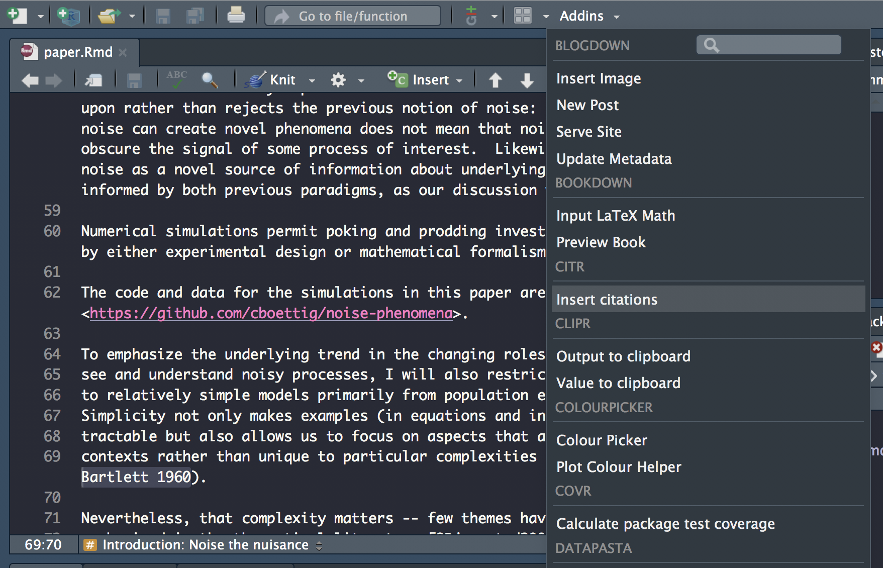

3. Search for citation to insert

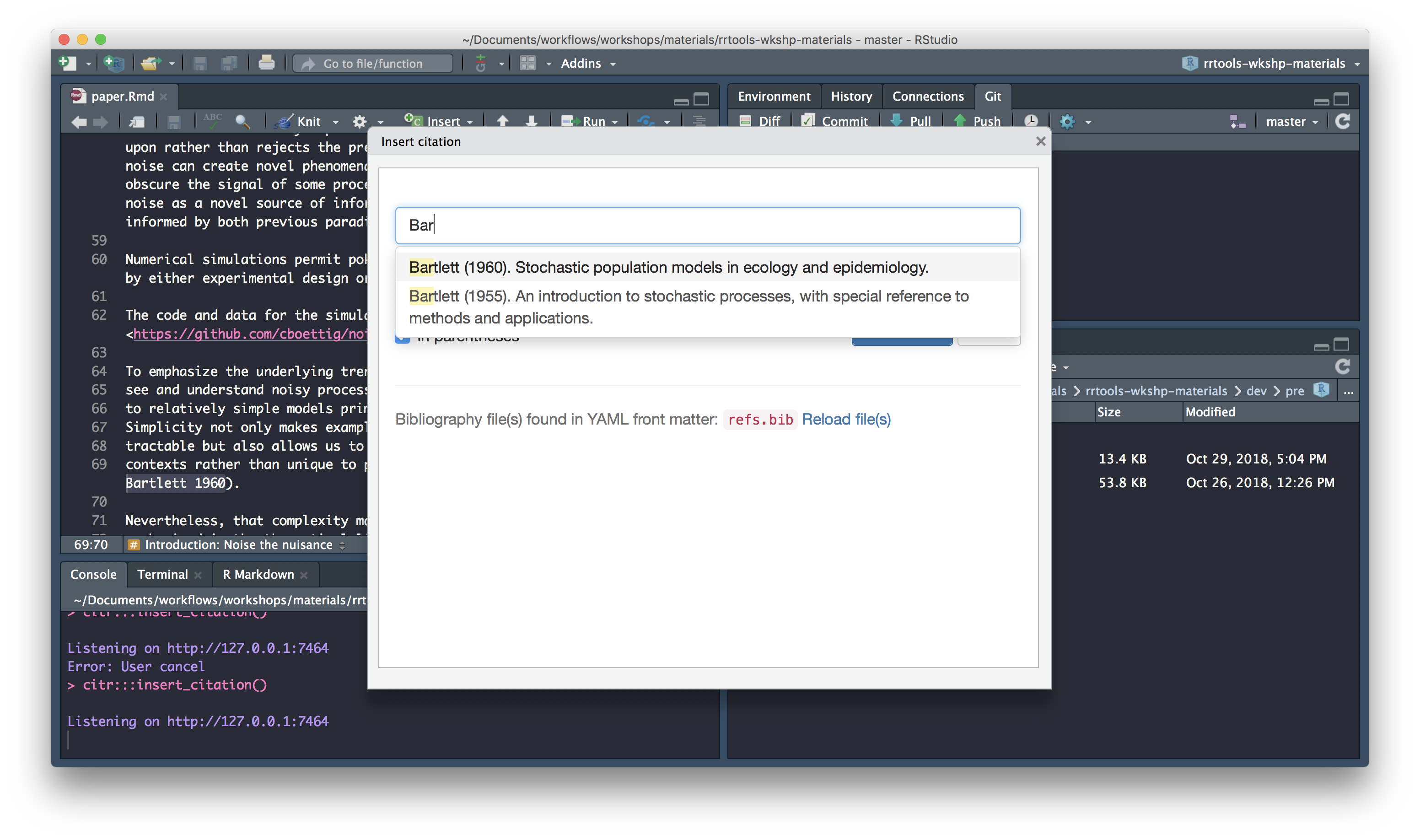
4. Select citation to insert

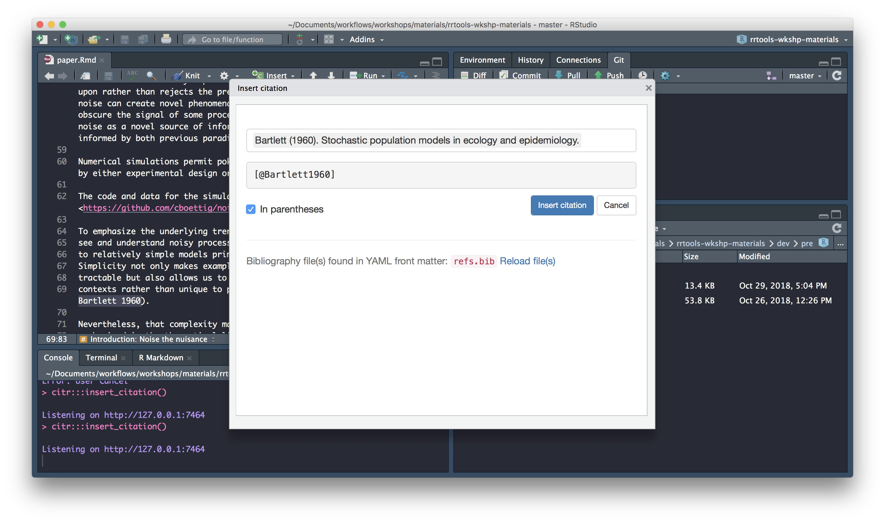
5. Insert citation

Carry on updating the rest of the citations. Don’t forget to check the abstract for citations!

🚦 Update math

For the sake of time today, and not to open this topic too deeply here, I’ve included the following LaTex equation syntax in the text:

\begin{align}
\frac{\mathrm{d} n}{\mathrm{d} t} = \underbrace{c n \left(1 - \frac{n}{N}\right)}_{\textrm{birth}} - \underbrace{e n}_{\textrm{death}}, \label{levins}
\end{align}

that generates equation 1 in the paper.pdf.

\[\begin{align} \frac{\mathrm{d} n}{\mathrm{d} t} = \underbrace{c n \left(1 - \frac{n}{N}\right)}_{\textrm{birth}} - \underbrace{e n}_{\textrm{death}}, \label{levins} \end{align}\]

So you don’t need to edit anything here.

Check Math expressions and Markdown extensions by bookdown for more information.

update inline math

Inline LaTeX equations and parameters can be written between a pair of dollar signs using the LaTeX syntax, e.g., $f(x) = 1/x$ generates \(f(x) = 1/x\).

Using paper.pdf to identify mathematical expressions in the text (generally they appear in italic), edit your paper.Rmd, enclosing them between dollar signs.

Check pdf output

Let’s knit our document to check our references and maths annotations have been updated correctly by clicking on the Knit tab.

---

🚦 Add code

Now that we’ve set up the text for our paper, let’s insert the code to generate figure 1.

Add libraries chunk

First let’s insert a libraries code chunk right at the top of the document to set up our analysis. Because it’s a setup chunk we set include = F which suppresses all output resulting from chunk evaluation.

```{r libraries, include=FALSE}
    
 ```

set document chunk options

Now, let’s set some knitr options for the whole document by adding the following code to our libraries chunk:

knitr::opts_chunk$set(echo = FALSE, message=FALSE, warning=FALSE, 
                      dev="cairo_pdf", fig.width=7, fig.height=3.5)

We’re setting default chunk options to:

• echo = FALSE
• message = FALSE
• warning = FALSE

to suppress code, warnings and messages in the output, and

• dev="cairo_pdf"
• fig.width=7
• fig.height=3.5

to specify how figures will appear.

add libraries

Copy and paste the code for loading all the libraries from analysis.R. Add library rrcompendium so we can access function recode_system_size. The libraries chunk should now look like so:

knitr::opts_chunk$set(echo = FALSE, message=FALSE, warning=FALSE, 
                      dev="cairo_pdf", fig.width=7, fig.height=3.5)

library(dplyr)
library(readr)
library(ggplot2)
library(ggthemes)
library(rrcompendium)

Add set-theme chunk

Right below the libraries chunk, insert a new chunk and call it set-theme

Copy the code to set the plot theme and pasted into the set-theme code:

theme_set(theme_grey())

Add figure1 chunk

Now scroll down towards the bottom of the document and create a new chunk just above the Conclusions section. Call it figure1

Add code

Copy and paste the remaining code into a new chunk which will create figure 1.

# create colour palette
colours <- ptol_pal()(2)

# load-data
data <- read_csv(here::here("gillespie.csv"), col_types = "cdiddd")  

# recode-data
data <- data %>% 
  mutate(system_size = recode(system_size, large = "A. 1000 total sites", small= "B. 100 total sites")) 

# plot-gillespie
data %>%
  ggplot(aes(x = time)) + 
  geom_hline(aes(yintercept = mean), lty=2, col=colours[2]) + 
  geom_hline(aes(yintercept = minus_sd), lty=2, col=colours[2]) + 
  geom_hline(aes(yintercept = plus_sd), lty=2, col=colours[2]) + 
  geom_line(aes(y = n), col=colours[1]) +
  facet_wrap(~system_size, scales = "free_y") 

🚦 Add caption

Finally, let’s update chunk figure1 to include a figure caption. The text for the caption is at the bottom of paper.txt. We can include it in the chunk header through chunk option fig.cap like so:

    ```{r figure1, figure1, fig.cap="Population dynamics from a Gillespie simulation of the Levins model with large (N=1000, panel A) and small (N=100, panel B) number of sites (blue) show relatively weaker effects of demographic noise in the bigger system. Models are otherwise identical, with e = 0.2 and c = 1 (code in appendix A). Theoretical predictions for mean and plus/minus one standard deviation shown in horizontal re dashed lines."} ```

---

Render final document to pdf

Let’s check our final work by re-knitting to pdf. You should be looking at something that looks a lot like paper.pdf

---

🚦 Add paper dependencies

Finally, before we’re finished, let’s ensure the dependencies introduced in the paper are included. We can use rrtools::add_dependencies_to_description()

rrtools::add_dependencies_to_description()

This function scans script files (.R, .Rmd, .Rnw, .Rpres, etc.) for external package dependencies indicated by library(), require() or :: and adds those packages to the Imports field in the package DESCRIPTION:

Imports: 
    bookdown,
    dplyr,
    ggplot2 (>= 3.0.0),
    ggthemes (>= 3.5.0),
    here (>= 0.1),
    knitr (>= 1.20),
    rticles (>= 0.6)
    

🔨 Install and Restart

Commit and push to GitHub!

Final compendium

You can see the resulting rrcompendium here

The complete compendium should contain the following files:

.
├── CONDUCT.md
├── CONTRIBUTING.md
├── DESCRIPTION
├── LICENSE
├── LICENSE.md
├── NAMESPACE
├── R
│   └── process-data.R
├── README.Rmd
├── README.md
├── analysis
│   ├── data
│   │   ├── DO-NOT-EDIT-ANY-FILES-IN-HERE-BY-HAND
│   │   ├── derived_data
│   │   └── raw_data
│   │       └── gillespie.csv
│   ├── figures
│   ├── paper
│   │   ├── elsarticle.cls
│   │   ├── mybibfile.bib
│   │   ├── numcompress.sty
│   │   ├── paper.Rmd
│   │   ├── paper.fff
│   │   ├── paper.pdf
│   │   ├── paper.spl
│   │   ├── paper.tex
│   │   ├── paper_files
│   │   │   └── figure-latex
│   │   │       └── figure1-1.pdf
│   │   └── refs.bib
│   └── templates
│       ├── journal-of-archaeological-science.csl
│       ├── template.Rmd
│       └── template.docx
├── inst
│   └── testdata
│       └── gillespie.csv
├── man
│   └── recode_system_size.Rd
├── rrcompendium.Rproj
└── tests
    ├── testthat
    │   └── test-process-data.R
    └── testthat.R