Managing Dependencies
One of the most important aspects of reproducible research is managing dependencies.
For your analysis to run, it interacts with:
Operating system: The operating system of your computer.
System configurations: such as locations of libraries and the search path your computer uses to find files and libraries
System Level libraries. These are non-R libraries that R or packages in R you might be using depend on. (for example libraries such as
GEOS,GDALandPROJ4that geospatial R packages likesfandrgeosdepend on). Such external dependencies to R are listed asSystem Requirementsin R packageDESCRIPTIONfiles (e.g have a look at the relevant line in thesfpackageDESCRIPTION.R and the R packages your analysis depends on. For example, the version of R we’ve been using as well as packages
ggplot2anddplyr.
When someone else tries to reproduce your analysis on a different computer, if any of these elements differ from what existed on your own system when you last ran your analysis, e.g some of the dependencies are missing, different versions are available or code behaves differently on a different operating system, they may not be able to reproduce your work.
Managing R dependencies.
Your first consideration should be to ensure you retain information and ideally a way of automatically installing any R package dependencies your code depends on.
As there is no way to automatically install external system dependencies, you should highlight any such dependencies in your README and ideally provide installation instructions (or links to them). Have a look at the installation section of the documentation for package sf.
Minimal approach
Including Session Information
At the very minimum you could list the packages used in an analysis using sessionInfo() at the bottom of an .Rmd file. This however is not so useful for .R scripts (unless you save the output of the function to a separate file). It also doesn’t provide executable code for someone else to install the requirements.
Including an install.R script
A more convenient but still not very robust method of managing R dependencies would be to include an executable install.R script (like the one I’ve included for setting up the projects in this course on your local machine) which contains the commands to install all the required dependencies.
Here’s the example of install.R used to set up the wood-survey project
dependencies <- c("assertr", "checkmate", "cowsay", "data.table",
                  "dataspice", "devtools", "DT", "fs", "gapminder", "geosphere",
                  "ggthemes", "gitcreds", "glue", "here", "janitor", "jsonlite",
                  "knitr", "leaflet", "listviewer", "magrittr", "plotly", "raster",
                  "reprex", "rmarkdown", "sf", "skimr", "sloop",
                  "spData", "stringr", "testthat", "tidyr", "tidyverse", "tmap",
                  "usethis", "vroom")

# install CRAN dependencies
install.packages(dependencies)

# install github dependencies
devtools::install_github("hadley/emo")
The problem with this is that the versions of packages are not fixed. Instead, each time the script is run, the most up to date versions of packages are installed, and R also prompts you to update any packages already installed. Changes in packages and a general mismatch of versions compared to those used to develop the original code, could cause problems in code execution.
In the case of this book, I want the materials to work with up to date versions of packages. If there are problems with newer versions, I can correct the materials before I run the course. However, for a published analysis, using code you don’t plan to further develop (and therefore do not require that it tracks the evolution of packages in the R ecosystem), it would be better to be able to pin exact versions of packages. That way you can ensure another user will be working with the exact same versions of your dependencies.
Robust approach
Managing R dependencies with renv
The renv package is a new effort to bring project-local R dependency
management to your projects.
Underlying the philosophy of renv is that any of your existing workflows
should just work as they did before – renv helps manage library paths (and
other project-specific state) to help isolate your project’s R dependencies.
renv Workflow
The general workflow when working with renv is:
Call
renv::init()to initialize a new project-local environment with a private R library,Work in the project as normal, installing and removing new R packages as they are needed in the project,
Call
renv::snapshot()to save the state of the project library to the lockfile (calledrenv.lock),Continue working on your project, installing and updating R packages as needed.
Call
renv::snapshot()again to save the state of your project library if your attempts to update R packages were successful, or callrenv::restore()to revert to the previous state as encoded in the lockfile if your attempts to update packages introduced some new problems.
The renv::init() function attempts to ensure the newly-created project
library includes all R packages currently used by the project. It does this
by crawling R files within the project for dependencies with the
renv::dependencies() function. The discovered packages are then installed
into the project library with the renv::hydrate() function, which will also
attempt to save time by copying packages from your user library (rather than
re-installing from CRAN) as appropriate.
Calling renv::init() will also write out the infrastructure necessary to
automatically load and use the private library for new R sessions launched
from the project root directory. This is accomplished by creating (or amending)
a project-local .Rprofile with the necessary code to load the project when
the R session is started.
The following files are written to and used by projects using renv:
| File | Usage |
|---|---|
.Rprofile |
Used to activate renv for new R sessions launched in the project. |
renv.lock |
The lockfile, describing the state of your project’s library at some point in time. |
renv/activate.R |
The activation script run by the project .Rprofile. |
renv/library |
The private project library. |
Reproducibility with renv
Using renv, it’s possible to “save” and “load” the state of your project
library. More specifically, you can use:
renv::snapshot()to save the state of your project torenv.lock; andrenv::restore()to restore the state of your project fromrenv.lock.
For each package used in your project, renv will record the package version,
and (if known) the external source from which that package can be retrieved.
renv::restore() uses that information to retrieve and re-install those
packages in your project.
Using renv in our wood-survey project
Let’s go back into our wood-survey project and capture our dependencies into a project level R package library. We do this by first initialising renv
renv::init()* Initializing project ...
* Discovering package dependencies ... Done!
* Copying packages into the cache ... [99/99] Done!
The following package(s) will be updated in the lockfile:
# CRAN ===============================
- MASS [* -> 7.3-53]
- Matrix [* -> 1.2-18]
- lattice [* -> 0.20-41]
- mgcv [* -> 1.8-33]
- nlme [* -> 3.1-149]
# RSPM ===============================
- BH [* -> 1.75.0-0]
- DT [* -> 0.18]
- EML [* -> 2.0.5]
- R6 [* -> 2.5.0]
- RColorBrewer [* -> 1.1-2]
- Rcpp [* -> 1.0.6]
- V8 [* -> 3.4.1]
- assertr [* -> 2.8]
- backports [* -> 1.2.1]
- base64enc [* -> 0.1-3]
- broom [* -> 0.7.6]
- bslib [* -> 0.2.4]
- cachem [* -> 1.0.4]
- checkmate [* -> 2.0.0]
- cli [* -> 2.5.0]
- clipr [* -> 0.7.1]
- colorspace [* -> 2.0-0]
- commonmark [* -> 1.7]
- cpp11 [* -> 0.2.7]
- crayon [* -> 1.4.1]
- crosstalk [* -> 1.1.1]
- curl [* -> 4.3]
- dataspice [* -> 1.0.0]
- digest [* -> 0.6.27]
- dplyr [* -> 1.0.5]
- ellipsis [* -> 0.3.1]
- emld [* -> 0.5.1]
- evaluate [* -> 0.14]
- fansi [* -> 0.4.2]
- farver [* -> 2.1.0]
- fastmap [* -> 1.1.0]
- fs [* -> 1.5.0]
- generics [* -> 0.1.0]
- geosphere [* -> 1.5-10]
- ggplot2 [* -> 3.3.3]
- glue [* -> 1.4.2]
- gtable [* -> 0.3.0]
- here [* -> 1.0.1]
- highr [* -> 0.9]
- hms [* -> 1.0.0]
- htmltools [* -> 0.5.1.1]
- htmlwidgets [* -> 1.5.3]
- httpuv [* -> 1.6.0]
- isoband [* -> 0.2.4]
- janitor [* -> 2.1.0]
- jqr [* -> 1.2.0]
- jquerylib [* -> 0.1.4]
- jsonld [* -> 2.2]
- jsonlite [* -> 1.7.2]
- knitr [* -> 1.33]
- labeling [* -> 0.4.2]
- later [* -> 1.2.0]
- lazyeval [* -> 0.2.2]
- lifecycle [* -> 1.0.0]
- listviewer [* -> 3.0.0]
- lubridate [* -> 1.7.10]
- magrittr [* -> 2.0.1]
- markdown [* -> 1.1]
- mime [* -> 0.10]
- munsell [* -> 0.5.0]
- pillar [* -> 1.6.0]
- pkgconfig [* -> 2.0.3]
- promises [* -> 1.2.0.1]
- purrr [* -> 0.3.4]
- rappdirs [* -> 0.3.3]
- readr [* -> 1.4.0]
- renv [* -> 0.13.2]
- repr [* -> 1.1.3]
- rhandsontable [* -> 0.3.7]
- rlang [* -> 0.4.10]
- rmarkdown [* -> 2.7]
- rprojroot [* -> 2.0.2]
- sass [* -> 0.3.1]
- scales [* -> 1.1.1]
- shiny [* -> 1.6.0]
- skimr [* -> 2.1.3]
- snakecase [* -> 0.11.0]
- sourcetools [* -> 0.1.7]
- sp [* -> 1.4-5]
- stringi [* -> 1.5.3]
- stringr [* -> 1.4.0]
- tibble [* -> 3.1.1]
- tidyr [* -> 1.1.3]
- tidyselect [* -> 1.1.0]
- tinytex [* -> 0.31]
- utf8 [* -> 1.2.1]
- uuid [* -> 0.1-4]
- vctrs [* -> 0.3.7]
- viridisLite [* -> 0.4.0]
- whisker [* -> 0.4]
- withr [* -> 2.4.2]
- xfun [* -> 0.22]
- xml2 [* -> 1.3.2]
- xtable [* -> 1.8-4]
- yaml [* -> 2.2.1]
* Lockfile written to '/cloud/project/renv.lock'.
Restarting R session...
* Project '/cloud/project' loaded. [renv 0.13.2]Our project now also contains the infrastructure that powers renv dependency management:
.
├── .Rprofile
├── renv
│   ├── .gitignore
│   ├── activate.R
│   ├── library
│   │   └── R-4.0
│   ├── local
│   └── settings.dcf
└── renv.lock
The renv.lock contains a list of names and versions of packages used in our project.
The folder renv/library/R-4.0 contains the project specific library of installed packages for the R version the analysis is currently being performed on. This is never committed to git (it is by default ignored). Rather, we commit the rest of the files (renv.lock file, the .Rprofile file and the renv/activate.R). Making these available means others users of your code will have the appropriate packages installed in their own local library when the download and use your code.
So let’s commit all the files renv::init() created
Finally, if you carry on working on your analysis and install new packages, call renv::snapshot() to save the state of the project library.
Advanced - Capturing computational environments
What we’ve discussed above only relates to managing R package dependencies. As mentioned though, problems can also arise form differences in the wider computational environment (operating system, system libraries, system configurations, version of R).
More robust ways of capturing computational environments can be achieved through using technologies like Docker containers or services like Binder.
Docker
standardized units of software that package up everything needed to run an application: code, runtime, system tools, system libraries and settings in a lightweight, standalone, executable package
Docker containers allow a researcher to package up a project with all of the parts it needs - such as libraries, dependencies, and system settings - and ship it all out as one package.
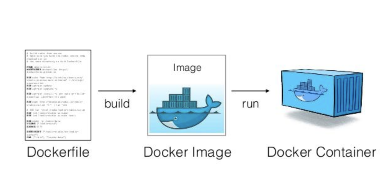
Dockerfile: Text file containing recipe for setting up computation environment.
Docker Image: Executable built from the Dockerfile with all required dependencies installed. Can have many images from the same
Dockerfile.Docker Container: Docker Images become containers at runtime
For a detailed discussion of the elements of a reproducible analysis and a more advanced example of how to use docker to capture them, have a look at the dependency chapter in the A Reproducible Research Compendium ebook or the Containers chapter in the Turing Way. There’s also a paper on Using Docker Containers to Improve Reproducibility in Software Engineering Research
package containerit
Also, check out package containerit which relies on Docker and automatically generates a container Dockerfile, or “recipe”, with setup instructions to recreate a runtime environment based on a given R session, R script, R Markdown file or workspace directory.
Binder
The mybinder service turn a Git repo into a collection of interactive notebooks or can even launch Rstudio in the cloud! Check out this video to find out more about how it works.
](assets/binder_comic.png)
Figure 2: Fig. 23 Figure credit: Juliette Taka, Logilab and the OpenDreamKit project
To learn more about binder and how to prepare projects to run on the service, have a look at the Turing Way chapter on Binder and the From Zero to Binder in R! tutorial.
ALso, check out package holepunch on GitHub for making your projects Binder ready.